June 8, 2022 | 6 min Read

Face Detection using MTCNN

MTCNN is a python (pip) library written by Github user ipacz , which implements the [paper Zhang, Kaipeng et al. “Joint Face Detection and Alignment Using Multitask Cascaded Convolutional Networks.” IEEE Signal Processing Letters 23.10 (2016): 1499–1503. Crossref. Web](https://arxiv.org/abs/1604.02878%5D(https://arxiv.org/abs/1604.02878%20%22https://arxiv.org/abs/1604.02878) .

In this paper, they propose a deep cascaded multi-task framework using different features of “sub-models” to each boost their correlating strengths.

MTCNN performs quite fast on a CPU, even though S3FD is still quicker running on a GPU – but that is a topic for another post.

This post uses code from the following two sources, check them out, they are interesting as well:

Basic usage of MTCNN

Feel free to access the whole notebook via:

https://github.com/JustinGuese/mtcnn-face-extraction-eyes-mouth-nose-and-speeding-it-up

git clone https://github.com/JustinGuese/mtcnn-face-extraction-eyes-mouth-nose-and-speeding-it-up

Luckily MTCNN is available as a pip package, meaning we can easily install it using

pip install mtcnn

Now switching to Python/Jupyter Notebook we can check the installation with an import and quick verification:

import mtcnn
# print version
print(mtcnn.__version__)

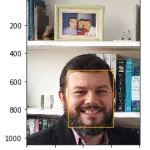
Afterwards, we are ready to load out test image using the matplotlib imread function .

import matplotlib.pyplot as plt
# load image from file
filename = "glediston-bastos-ZtmmR9D_2tA-unsplash.webp"
pixels = plt.imread(filename)
print("Shape of image/array:",pixels.shape)
imgplot = plt.imshow(pixels)
plt.show()

Now your output will look a lot like this:

{'box': [1942, 716, 334, 415], 'confidence': 0.9999997615814209, 'keypoints': {'left_eye': (2053, 901), 'right_eye': (2205, 897), 'nose': (2139, 976), 'mouth_left': (2058, 1029), 'mouth_right': (2206, 1023)}}
{'box': [2084, 396, 37, 46], 'confidence': 0.9999206066131592, 'keypoints': {'left_eye': (2094, 414), 'right_eye': (2112, 414), 'nose': (2102, 426), 'mouth_left': (2095, 432), 'mouth_right': (2112, 431)}}
{'box': [1980, 381, 44, 59], 'confidence': 0.9998701810836792, 'keypoints': {'left_eye': (1997, 404), 'right_eye': (2019, 407), 'nose': (2010, 417), 'mouth_left': (1995, 425), 'mouth_right': (2015, 427)}}
{'box': [2039, 395, 39, 46], 'confidence': 0.9993435740470886, 'keypoints': {'left_eye': (2054, 409), 'right_eye': (2071, 415), 'nose': (2058, 422), 'mouth_left': (2048, 425), 'mouth_right': (2065, 431)}}

What does this tell us? A lot of it is self-explanatory, but it basically returns coordinates, or the pixel values of a rectangle where the MTCNN algorithm detected faces. The “box” value above returns the location of the whole face, followed by a “confidence” level.

If you want to do more advanced extractions or algorithms, you will have access to other facial landmarks, called “keypoints” as well. Namely the MTCNN model located the eyes, mouth and nose as well!

Drawing a box around faces

To demonstrate this even better let us draw a box around the face using matplotlib:

# draw an image with detected objects
def draw_facebox(filename, result_list):
# load the image
data = plt.imread(filename)
# plot the image
plt.imshow(data)
# get the context for drawing boxes
ax = plt.gca()
# plot each box
for result in result_list:
# get coordinates
x, y, width, height = result['box']
# create the shape
rect = plt.Rectangle((x, y), width, height, fill=False, color='green')
# draw the box
ax.add_patch(rect)
# show the plot
plt.show()

# filename = 'test1.webp' # filename is defined above, otherwise uncomment
# load image from file
# pixels = plt.imread(filename) # defined above, otherwise uncomment
# detector is defined above, otherwise uncomment
#detector = mtcnn.MTCNN()
# detect faces in the image
faces = detector.detect_faces(pixels)
# display faces on the original image
draw_facebox(filename, faces)

Displaying eyes, mouth, and nose around faces

Now let us take a look at the aforementioned “keypoints” that the MTCNN model returned.

We will now use these to graph the nose, mouth, and eyes as well.
We will add the following code snippet to our code above:

# draw the dots
for key, value in result['keypoints'].items():
# create and draw dot
dot = plt.Circle(value, radius=20, color='orange')
ax.add_patch(dot)

With the full code from above looking like this:

# draw an image with detected objects
def draw_facebox(filename, result_list):
# load the image
data = plt.imread(filename)
# plot the image
plt.imshow(data)
# get the context for drawing boxes
ax = plt.gca()
# plot each box
for result in result_list:
# get coordinates
x, y, width, height = result['box']
# create the shape
rect = plt.Rectangle((x, y), width, height,fill=False, color='orange')
# draw the box
ax.add_patch(rect)
# draw the dots
for key, value in result['keypoints'].items():
# create and draw dot
dot = plt.Circle(value, radius=20, color='red')
ax.add_patch(dot)
# show the plot
plt.show()

# filename = 'test1.webp' # filename is defined above, otherwise uncomment
# load image from file
# pixels = plt.imread(filename) # defined above, otherwise uncomment
# detector is defined above, otherwise uncomment
#detector = mtcnn.MTCNN()
# detect faces in the image
faces = detector.detect_faces(pixels)
# display faces on the original image
draw_facebox(filename, faces)

Advanced MTCNN: Speed it up (\~x100)!

Now let us come to the interesting part. If you are going to process millions of pictures you will need to speed up MTCNN, otherwise, you will either fall asleep or your CPU will burn before it will be done.

But what exactly are we talking about? If you are running the above code it will take around one second, meaning we will process around one picture per second. If you are running MTCNN on a GPU and use the sped-up version it will achieve around 60-100 pictures/frames a second. That is a boost of up to 100 times!

If you are for example going to extract all faces of a movie, where you will extract 10 faces per second (one second of the movie has on average around 24 frames, so every second frame) it will be 10 * 60 (seconds) * 120 (minutes) = 72,000 frames.

Meaning if it takes one second to process one frame it will take 72,000 * 1 (seconds) = 72,000s / 60s = 1,200m = 20 hours

With the sped-up version of MTCNN this task will take 72,000 (frames) / 100 (frames/sec) = 720 seconds = 12 minutes!

To use MTCNN on a GPU you will need to set up CUDA, cudnn, pytorch and so on. Pytorch wrote a good tutorial about that part .

Once installed we will do the necessary imports as follows:

from facenet_pytorch import MTCNN
from PIL import Image
import torch
from imutils.video import FileVideoStream
import cv2
import time
import glob
from tqdm.notebook import tqdm

device = 'cuda' if torch.cuda.is_available() else 'cpu'

filenames = ["glediston-bastos-ZtmmR9D_2tA-unsplash.webp","glediston-bastos-ZtmmR9D_2tA-unsplash.webp"]

See how we defined the device in the code above? You will be able to run everything on a CPU as well if you do not want or can set up CUDA.

Next, we will define the extractor:

# define our extractor
fast_mtcnn = FastMTCNN(
stride=4,
resize=0.5,
margin=14,
factor=0.6,
keep_all=True,
device=device
)

In this snippet, we pass along some parameters, where we for example only use half of the image size, which is one of the main impact factors for speeding it up.

And finally, let us run the face extraction script:

def run_detection(fast_mtcnn, filenames):
frames = []
frames_processed = 0
faces_detected = 0
batch_size = 60
start = time.time()

for filename in tqdm(filenames):

v_cap = FileVideoStream(filename).start()
v_len = int(v_cap.stream.get(cv2.CAP_PROP_FRAME_COUNT))

for j in range(v_len):

frame = v_cap.read()
frame = cv2.cvtColor(frame, cv2.COLOR_BGR2RGB)
frames.append(frame)

if len(frames) >= batch_size or j == v_len - 1:

faces = fast_mtcnn(frames)

frames_processed += len(frames)
faces_detected += len(faces)
frames = []

print(
f'Frames per second: {frames_processed / (time.time() - start):.3f},',
f'faces detected: {faces_detected}\r',
end=''
)

v_cap.stop()

run_detection(fast_mtcnn, filenames)

The above image shows the output of the code running on an NVIDIA Tesla P100, so depending on the source material, GPU and processor you might experience better or worse performance.

[Are you working on a similar project? Are you interested in something similar? [contact us](/contact) now for a free 15-minute consultation.](/contact/)

Justin Guese

Justin Güse